Keras Visualization Toolkit

keras-vis is a high-level toolkit for visualizing and debugging your trained keras neural net models. Currently supported visualizations include:

Activation maximization
Saliency maps
Class activation maps

All visualizations by default support N-dimensional image inputs. i.e., it generalizes to N-dim image inputs to your model.

The toolkit generalizes all of the above as energy minimization problems with a clean, easy to use, and extendable interface. Compatible with both theano and tensorflow backends with 'channels_first', 'channels_last' data format.

Quick links

Read the documentation at https://raghakot.github.io/keras-vis.
- The Japanese edition is https://keisen.github.io/keras-vis-docs-ja.
Join the slack channel for questions/discussions.
We are tracking new features/tasks in waffle.io. Would love it if you lend us a hand and submit PRs.

Getting Started

In image backprop problems, the goal is to generate an input image that minimizes some loss function. Setting up an image backprop problem is easy.

Define weighted loss function

Various useful loss functions are defined in losses. A custom loss function can be defined by implementing Loss.build_loss.

from vis.losses import ActivationMaximization
from vis.regularizers import TotalVariation, LPNorm

filter_indices = [1, 2, 3]

# Tuple consists of (loss_function, weight)
# Add regularizers as needed.
losses = [
    (ActivationMaximization(keras_layer, filter_indices), 1),
    (LPNorm(model.input), 10),
    (TotalVariation(model.input), 10)
]

Configure optimizer to minimize weighted loss

In order to generate natural looking images, image search space is constrained using regularization penalties. Some common regularizers are defined in regularizers. Like loss functions, custom regularizer can be defined by implementing Loss.build_loss.

from vis.optimizer import Optimizer

optimizer = Optimizer(model.input, losses)
opt_img, grads, _ = optimizer.minimize()

Concrete examples of various supported visualizations can be found in examples folder.

Installation

1) Install keras with theano or tensorflow backend. Note that this library requires Keras > 2.0

2) Install keras-vis

From sources

sudo python setup.py install

PyPI package

sudo pip install keras-vis

Visualizations

NOTE: The links are currently broken and the entire documentation is being reworked. Please see examples/ for samples.

Neural nets are black boxes. In the recent years, several approaches for understanding and visualizing Convolutional Networks have been developed in the literature. They give us a way to peer into the black boxes, diagnose mis-classifications, and assess whether the network is over/under fitting.

Guided backprop can also be used to create trippy art, neural/texture style transfer among the list of other growing applications.

Various visualizations, documented in their own pages, are summarized here.

Conv filter visualization

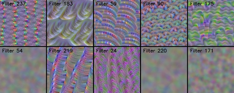
Convolutional filters learn 'template matching' filters that maximize the output when a similar template pattern is found in the input image. Visualize those templates via Activation Maximization.

Dense layer visualization

How can we assess whether a network is over/under fitting or generalizing well?

Attention Maps

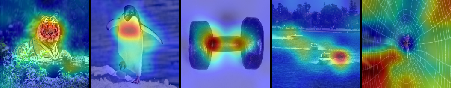
How can we assess whether a network is attending to correct parts of the image in order to generate a decision?

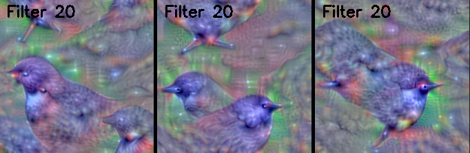
Generating animated gif of optimization progress

It is possible to generate an animated gif of optimization progress by leveraging callbacks. Following example shows how to visualize the activation maximization for 'ouzel' class (output_index: 20).

from vis.losses import ActivationMaximization
from vis.regularizers import TotalVariation, LPNorm
from vis.modifiers import Jitter
from vis.optimizer import Optimizer

from vis.callbacks import GifGenerator
from vis.utils.vggnet import VGG16

# Build the VGG16 network with ImageNet weights
model = VGG16(weights='imagenet', include_top=True)
print('Model loaded.')

# The name of the layer we want to visualize
# (see model definition in vggnet.py)
layer_name = 'predictions'
layer_dict = dict([(layer.name, layer) for layer in model.layers[1:]])
output_class = [20]

losses = [
    (ActivationMaximization(layer_dict[layer_name], output_class), 2),
    (LPNorm(model.input), 10),
    (TotalVariation(model.input), 10)
]
opt = Optimizer(model.input, losses)
opt.minimize(max_iter=500, verbose=True, image_modifiers=[Jitter()], callbacks=[GifGenerator('opt_progress')])

Notice how the output jitters around? This is because we used Jitter, a kind of ImageModifier that is known to produce crisper activation maximization images. As an exercise, try:

Without Jitter
Varying various loss weights

opt_progress

Citation

Please cite keras-vis in your publications if it helped your research. Here is an example BibTeX entry:

@misc{raghakotkerasvis,
  title={keras-vis},
  author={Kotikalapudi, Raghavendra and contributors},
  year={2017},
  publisher={GitHub},
  howpublished={\url{https://github.com/raghakot/keras-vis}},
}