Baking rotational invariance into a neuron

This is a continuation from the first post on exploring alternative neural computational models. To recap quickly, a neuron is fundamentally acting as a pattern matching unit by computing the dot product \(W \cdot X\), which is equivalent to unnormalized cosine similarity between vectors \(W\) and \(X\).

This model of pattern matching is very naive, in a sense that it is not invariant to translations or rotations. Consider the following weight vector template (conv filter) corresponding to vertical edge pattern |

\(W = \begin{bmatrix} 0.2 & 1.0 & 0.2\\ 1.0 & 1.0 & 1.0\\ 0.2 & 1.0 & 0.2 \end{bmatrix} \)

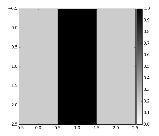
Figure 1. Visual representation of \(W\) template

When a neuron tries to match this pattern in a \(3 \times 3\) input image patch, it will only output a high value if a vertical edge is found in the center of the image patch. i.e., dot product is not invariant to shifts. My first thought was to use Pearson coefficient as it provides shift invariance. However, this not a problem in practice as the filter is slid across all possible \(3 \times 3\) patches within the input image (see fig2).

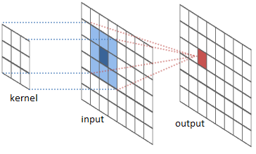
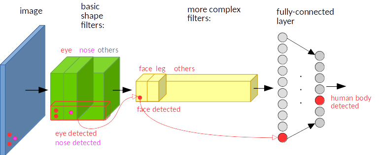
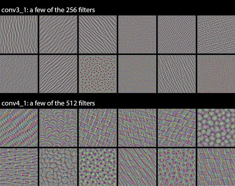
Figure 2. Sliding filter over input image to generate the output activation area (image borrowed from river trail documentation)

In a way, the sliding window operation is quite clever as it communicates information about parts of the image matching filter template without increasing the number of trainable parameters. As a concrete example, consider a conv-net with filters as shown in fig3^[1]. The first layer filters (green) detect eyes, nose etc., second layer filters (yellow) detect face, leg etc., by aggregating features from first layer and so on^[2].

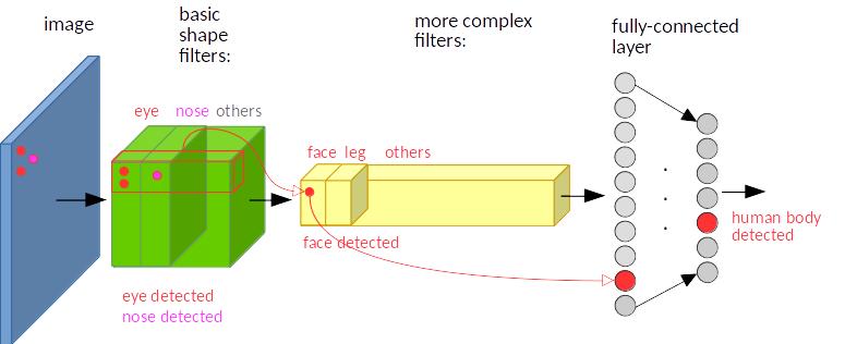
Figure 3. Hypothetical conv-net filters to illustrate how a human might be detected. (image borrowed from quora post)

Now suppose the face (represented by two red and one magenta point) is moved to another corner as shown in fig4. The same activations occur, leading to the same end result.

Figure 4. Illustration of activations when an input object is shifted. (image borrowed from quora post)

So far so good. How about rotational invariance? We know that a lot of learned conv filters are identical, but rotated by some non-random factor. Instead of learning rotational invariance in this manner, we will try to build it directly into the computational model. The motivation is simple - the neuron should output high value even if some rotated version of pattern is present in the input. Hopefully this eliminates redundant filters and improves test time accuracy.

Figure 5. A few conv filters of a vggnet (image borrowed from keras blog post). Notice how some filters are identical but rotated.

Endowing rotational invariance

How can we build rotational invariance into dot product similarity computation? After searching for a bit on the Internet, I couldn’t find any obvious similarity metrics that do this. Sure there is SIFT and SURF, but they are complex computations and cannot be expressed in terms of dot products alone.

Instead of trying to come up with a metric, I decided to try the brute force approach of matching the input patch with all possible rotations of the filter. If we take max of all those outputs, then, in principle, we are choosing the output resulting from the rotated filter that best aligns with the pattern in input patch. This strategy is partly inspired by how conv nets gets around translational invariance problem by simply sliding the filter over all possible locations. Unlike sliding operation, which is an architectural property rather than the computational property of the neuron, the brute force rotations of filters can be confined within the abstraction of neuron, making it a part of the computational model.

Lets look at this idea in more concrete terms. A neuron receives input \(X\) and has associated weights \(W\). Let \(r\) denote some arbitrary discrete rotation \(\theta\). Instead of directly computing \(W \cdot X\), we will compute \(\max \{ rW \cdot X, r^{2}W \cdot X, \cdots, r^{k}W \cdot X \}\), where \(k = \left \lceil \frac{360}{\theta} \right \rceil\) is the number of brute force rotations of \(\theta\) step.

This idea has a number of practical challenges.

How do we decide \(\theta\)? If we set \(\theta = 90^{\circ}\), we can produce 4 rotated filters.
For \(\theta \neq 90^{\circ}\) we need interpolation, which might change filter shape.

To avoid interpolation, we can try to shift the image by rotating elements clockwise from outermost layer to innermost layer. For a \(3 \times 3\) image, there are 8 possible rotations. Unfortunately, this only works for filters that are symmetric along the center of the matrix. As an example, consider all 8 rolled rotations of the L shaped filter (fig 6). As the image is not symmetric along the center, we get skewed representations for \(45\circ\) rotations. The second image in fig 6 still looks like an L, except that the tail end of L is squished upwards to maintain \(3 \times 3\) filter shape.

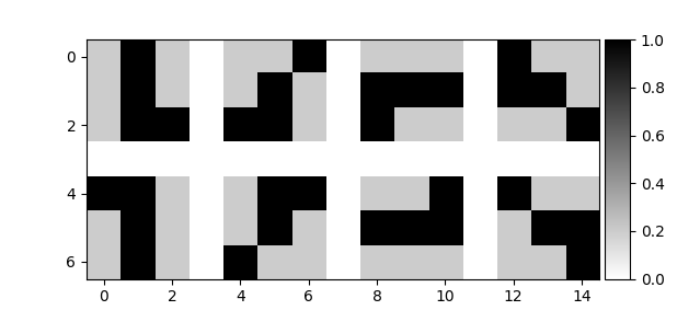
Figure 6. All 8 shifts of the L shaped filter. Each row contains a clockwise rolled elements from the previous.

Despite the setback, all \(90^{\circ}\) rotations are accurate and \(45^{\circ}\) rotations are only slightly skewed. Skew might be a blessing in disguise as it might endow the neuron to be deform invariant as well (wishful thinking). In either case, the deformations are not too bad for \(3 \times 3\) filters, and it is at-least worth experimenting with vggnet which uses all \(3 \times 3\) conv filters.

Alternatively, instead of trying all possible alignments, we could try to find \(\theta\) that maximizes the dot product.

Let R denote \(2 \times 2\) rotation matrix.

\(R = \begin{bmatrix} cos(\theta) & sin(\theta)\\ -sin(\theta) & cos(\theta) \end{bmatrix}\)

To accomplish optimal alignment, we need \(\theta\) such that:

\(\arg\max_\theta R_{\theta}W \cdot X\)

This can be solved by differentiating with respect to \(\theta\) and equating the derivative to 0.

I finally decided to go with the brute force approach to quickly test out the idea and maybe further develop the math for optimal alignment if it showed promise. The brute-force computations discussed so far apply to an individual neuron. For Convolutional layer, the output is generated as follows:

Generate all 8 rotated filters from \(W\), \(W_{1}, \cdots, W_{8}\).
Compute output activation volumes^[3] \(O_{1}, \cdots, O_{8}\) by convolving input with \(W_{1}, \cdots, W_{8}\).
Across volumes, select \(x, y\) value corresponding to filter \((row, col)\) that has the max value. This corresponding to selecting the best aligned filter with input patch across the 8 rotations.

These steps can be implemented as follows. Note that W.shape = (rows, cols, nb_input_filters, nb_output_filters). You also need bleeding edge tensorflow from master; as of Nov 2016, gather_nd does not have a gradient implementation.

import tensorflow as tf


# The clockwise shift-1 rotation permutation.
permutation = [[1, 0], [0, 0], [0, 1], [2, 0], [1, 1], [0, 2], [2, 1], [2, 2], [1, 2]]


def shift_rotate(w, shift=1):
    shape = w.get_shape()
    for i in range(shift):
        w = tf.reshape(tf.gather_nd(w, permutation), shape)
    return w


def conv2d(x, W, **kwargs):
    # Determine all 7 rotations of w.
    w = W
    w_rot = [w]
    for i in range(7):
        w = shift_rotate(w)
        w_rot.append(w)

    # Convolve with all 8 rotations and stack.
    outputs = tf.stack([tf.nn.conv2d(x, w_i, **kwargs) for w_i in w_rot])

    # Max filter activation across rotations.
    output = tf.reduce_max(outputs, 0)
    return output

Experimental Setup

The setup is as follows.

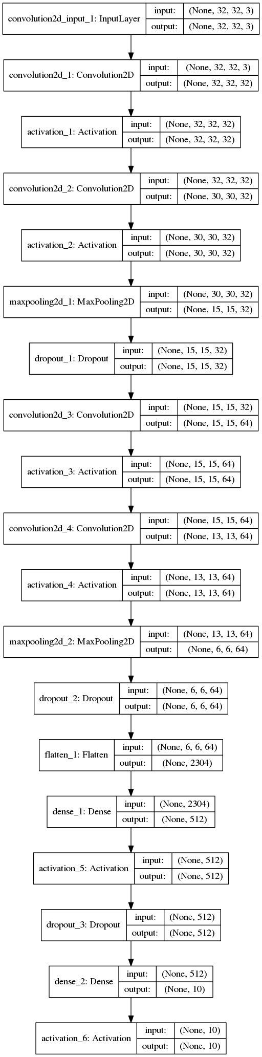
Mini vggnet (1,250,858 parameters) comprising of \(3 \times 3\) convolutions with ReLU activation.
cifar10 dataset augmented with 10% random shifts along image rows/cols along with a 50% chance of horizontal flip.
batch size = 32, epochs = 200 with early stopping.
Adam optimizer with initial learning rate of \(10^{-3}\), and reduced by a factor of \(10^{-1}\) when convergence stalls.
random_seed = 1337 for reproducibility.

Figure 7. Test model

Discussion

Disappointingly, rotational invariant model resulted in lower val accuracy than the baseline. I had three running hypothesis as to why this might happen.

Implementation issue. I ruled this out by testing the conv2d(…) implementation by feeding it numpy arrays and verifying the output.
Perhaps, rotational invariance is not a good idea for the earlier filters. As an example, consider a latter layer that uses vertical and horizontal edge features for the preceeding layer to detect a square like shape. Having rotational invariance means that it is not possible to distinguish horizontal from vertical edges, making square detection a lot more challenging.
Maybe the skew from \(\theta = \{45^{\circ}, 135^{\circ}, 225^{\circ}, 315^{\circ}\}\) was an issue after all.

To test 2, 3, I decided to run 6 more experiments by using:

Use new conv logic only on last 4, 3, 2, 1 layer(s). If hypothesis 2 is true, the convergence should get better.
Use \(90^{\circ}\) rotations (4 filters) and \(45^{\circ}\) rotations (8 filters) to test if skew introduced by the 8 filter version was really an issue.

The results of these experiments are summarized in fig 8.

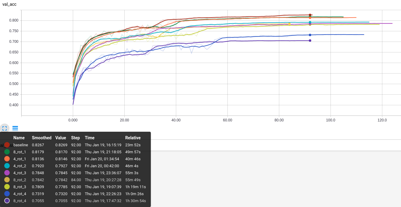
Figure 8. Convergence graphs for #{8/4 rotations}_rot_{last 1, 2, 3, 4 conv with new conv layer} and the baseline model. Models in legend are ordered in descending order of accuracy.

It seems evident that using rotationally invariant convolutional layers everywhere is not a good idea (4_rot_4 and 8_rot_4 have the lowest values). In line with hypothesis 2, the accuracy improved as we get rid of earlier rotationally invariant conv layers, with 4_rot_1 and 8_rot_1 on par/slightly better than the baseline model. The skew (according to hypothesis 3) does not seem to the issue as 8_rot_[4, 3, 2, 1] closely followed 4_rot_[4, 3, 2, 1] accuracies.

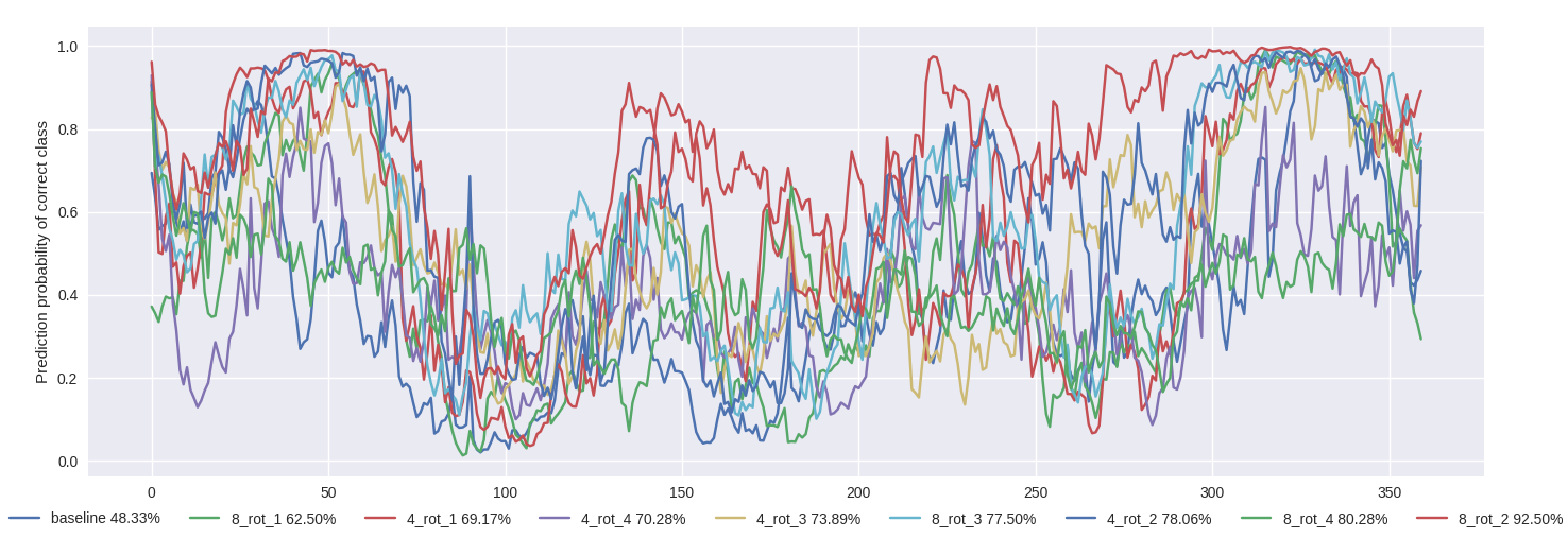
Since 4_rot_1 and 8_rot_4 converged to similar val_acc as the baseline, it is worth comparing how prediction probability of the correct class changes as we rotate the input image from \(\theta = \{0, 360\}\) by a step of \(1^{\circ}\). Fig 9. shows this comparison across all models for the sake of completeness. It is awesome to note that all models outperform baseline model in terms of rotational invariance.

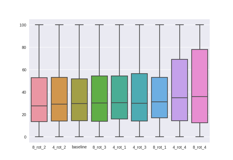
Figure 9. Prediction probability of the correct output class as a test input image is rotated from \(\theta = \{0, 360\}\) by step of \(1^{\circ}\) across models. Legend shows the percentage correct classifications across rotations (ascending order).

Instead of checking random images, lets compute these values for 1000 random test images and use a box plot to see mean, std, min, max of percentage correct classifications across all rotations. Interestingly, 8_rot_4, 4_rot_4 show the best rotational invariance (higher mean, large std in positive direction). It is also somewhat mysterious why 8_rot_2, 4_rot_2 is slightly worse than baseline compared to 1, 3, 4.

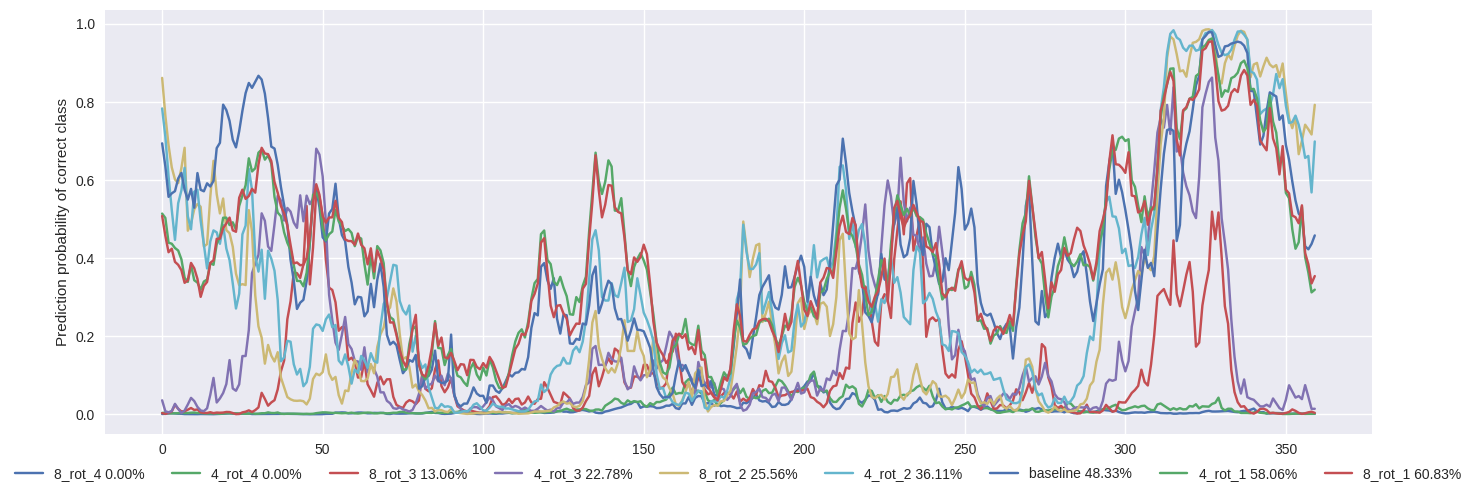
Figure 10. Box plot of percentage correct classifications across all rotations for 1000 random test images (in ascending order of mean).

Can we get the benefits of 8/4 rot models without the slower convergence? What if we applied new conv model (8/4 rotations) to the baseline model weights? Fig 11. shows the results for a single image. It is very curious to note that 8_rot_4 and 4_rot_4 models yield zero accuracy. This seems to indicate that weights from the usual conv layer won’t translate well into rotated conv model (the errors across various layers add up). The error rates seem to recover as we remove rotational conv layers from the early layers, but there is a lot of noise since this is for a single test image.

Figure 11. Prediction probability of the correct output class as a test input image is rotated from \(\theta = \{0, 360\}\) by step of \(1^{\circ}\) across models with baseline trained weights. Legend shows the percentage correct classifications across rotations (ascending order).

To get a clearer picture, lets compute the box plot by considering 1000 random test images as described earlier. Fig. 12 makes it pretty clear that we cannot just add rotation operations to a regular model after training. On the flip side, it provides evidence that rotational conv affects the weights.

Figure 12. Box plot of percentage correct classifications across all rotations for 1000 random test images (in ascending order of mean). Note that all models use trained baseline weights.

Conclusions

The code to reproduce all the experiments is available on Github. Feel free to reuse or improve.

Even though convergence is slower, 8 rotations seem to offer better invariance compared to 4 rotations. It would be interesting to see whether all models converge to the same accuracy eventually.
Filter skew does not seem to be an issue.
All models seem to exhibit the same seasonal pattern of accuracy with respect to rotation (see fig. 9). What’s with the weird dip at \(100^{\circ}\)?

EDITs

It might be worth experimenting by concatenating activations from rotated filters instead of max operation in light of recent success with DenseNets.
Try out squeeze net style feature compression following concatenation of rotated filters.

1. First layer filters generally detect basic lines and textures, this is just a simplified view to illustrate the point

2. In reality, convolution filters may detect objects that have no meaningful interpretation

3. If you are not familiar with the idea of activation volumes, I would recommend referring to CS231n Convolutional Neural Networks for Visual Recognition for an outstanding explanation.