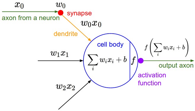
Despite different variations of neural networks architectures, the computational model of a neuron hasn’t changed since inception. Every neuron has \(n\) incoming inputs \(X = (x_{1}, x_{2}, …, x_{n})\) with weights \(W = (w_{1}, w_{2}, …, w_{n})\). A neuron then computes \(W.X = \sum_{i=0}^{n}w_{i}.x_{i}\), forwards it through some nonlinearity like sigmoid or ReLU to generate the output[1].
As far as i am aware, all architectures build on this fundamental computational model. Let us examine what the computation is conceptually doing in a step by step fashion.
-
Each input component \(x_{i}\) is being magnified or diminished when multiplied with a scaling factor \(w_{i}\). This can be interpreted as enhancing or diminishing the contribution of some pattern component \(x_{i}\) to the output decision. Think of these weights as knobs that range from \([-\infty, +\infty]\). The task of learning is to tune these knobs to the correct value.
-
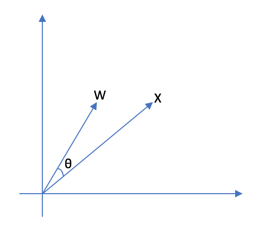
The computation \(W.X\) is then enhancing/diminishing various input components of vector \(X\). In terms of linear algebra, the dot product of \(W\) and \(X\) can be interpreted as computing similarity. Consider \(X = (x_{1}, x_{2})\) and \(W = (w_{1}, w_{2})\). If you imagine plotting these vectors on a 2D graph paper, \(\frac{W.X}{|W||X|}\) is the cosine of angle between these two vectors. When these two vectors align (point in the same direction), the value of \(W.X\) is maximized indicating high degree of similarity. From this point of view, neuron is fundamentally a pattern matching unit which outputs a large value when it matches a specific pattern (encoded by weights) in the input[2].
-
In a complex neural network, every neuron is matching the input against some template encoded via weights and forwarding that result to the subsequent layers. In case of image recognition, the first layer neurons might match whether the input contains vertical edge, horizontal edge and so on. The circle detection neuron might use various edge matching computation results from previous layers to detect the shape patterns.
So far so good. What is the purpose of activation function? To understand the motivation, consider the geometric perspective of the computation through the lens of linear algebra.
\( W.X = \begin{bmatrix} w_{1} \\ w_{2} \\ \vdots \\ w_{n} \end{bmatrix} \begin{bmatrix} x_{1} & x_{2} & \cdots & x_{n} \end{bmatrix} \)
Geometrically, this can be interpreted as a linear transformation of \(X\). Additionally, there is a bias term to shift the origin. So, the computation \(W.X + b\) can be interpreted as an affine transformation. Without an non-linear activation function, multiple linear transformations within each layer \(W_{L}\) can be condensed into a single layer with \(W = \prod_{L}W_{L}\). A single layered linear neural network is pretty limited in its representational power.
Lets put all this together to interpret what a multi-layered neural network might be doing[3]:
-
Suppose we input a \(100 \times 100\) image to a vggnet. The input tensor \(X\) can be thought of as a vector with 10000 basis. Each basis is representing some positional component in an image.
-
We know that the very first conv layer learns gabor filter like edge detection weight templates. Lets assume that the first convolutional layer filter generates \(100 \times 100\) output (assuming appropriate padding). This can be seen as transforming input from positional basis vector space to edge-like basis vector space. Instead of measuring the pixel intensity, the new vector space measures the similarity of the positional input patch with respect to a edge-detection templates (\(3 \times 3\) conv filter weights). Extrapolating on this notion, every layer transforms the data into a more meaningful basis vector space, eventually leading to basis vectors comprising of output categories.
Motivation
In the current computational model, the output of a neuron is different even though \(X\) and \(W\) perfectly align with each other but differ in magnitudes. As each \(w_{i}\) has range \([-\infty, \infty]\), backprop is essentially searching for this weight vector spanning all of the weight vector space.
If we view a neuron as fundamental template matching unit, then various magnitude (length) of \(X\) and \(W\) should yield the same output. If we constrain \(W\) to be a unit vector (\(|W| = 1\)), then backprop would only need to search along points on a hypersphere of unit radius. Although the hypersphere contains infinitely many points, with sufficient discretization, the search space intuitively feels a lot smaller than the entire weight vector space.
Considering that weight sharing (a form on constraint) in conv-nets led to huge improvements, constraining seems like a reasonable approach. Weight regularization - a form of constraint - penalizes large \(|W|\) and vaguely fits the idea of encouraging weight updates to explore points along the hypersphere.
I think that in general, constraining as a research direction is largely unexplored. For example, it might be interesting to try and constrain conv filters to be as distinct and diverse and possible. I will follow up on these investigations in a future blog.
Getting back to the topic at hand, there are several options for constraining \(|W| = 1\).
-
Penalize when \(|W|\) deviates from 1 as a regularization loss.
-
Represent \(W\) in parametric form. Each \(w_{i}\) can be calculated using n-dim spherical coordinates.
-
Instead of computing \(W.X\), compute \(\frac{W}{|W|} \times X\). Normalizing \(W\) ensures that the output does not change due to scaling. Consequently, the gradient of output with respect to \(W\) can only exist if \(W\) changes along the unit hypersphere.
Experimental Setup
I explored option 3 as it was the simplest to implement. The setup is as follows.
-
Mini vggnet (1,250,858 parameters) comprising of \(3 \times 3\) convolutions with ReLU activation.
-
cifar10 dataset augmented with 10% random shifts along image rows/cols along with a 50% chance of horizontal flip.
-
batch size = 32, epochs = 200 with early stopping.
-
Adam optimizer with initial learning rate of \(10^{-3}\), and reduced by a factor of \(10^{-1}\) when convergence stalls.
-
random_seed = 1337for reproducibility.
\(W_{norm}\) is calculated as:
# 1e-8 is used to prevent division by 0
W_norm = W / (tf.sqrt(tf.reduce_sum(tf.square(W), axis=[0, 1, 2], keep_dims=True)) + 1e-8)
Experiments
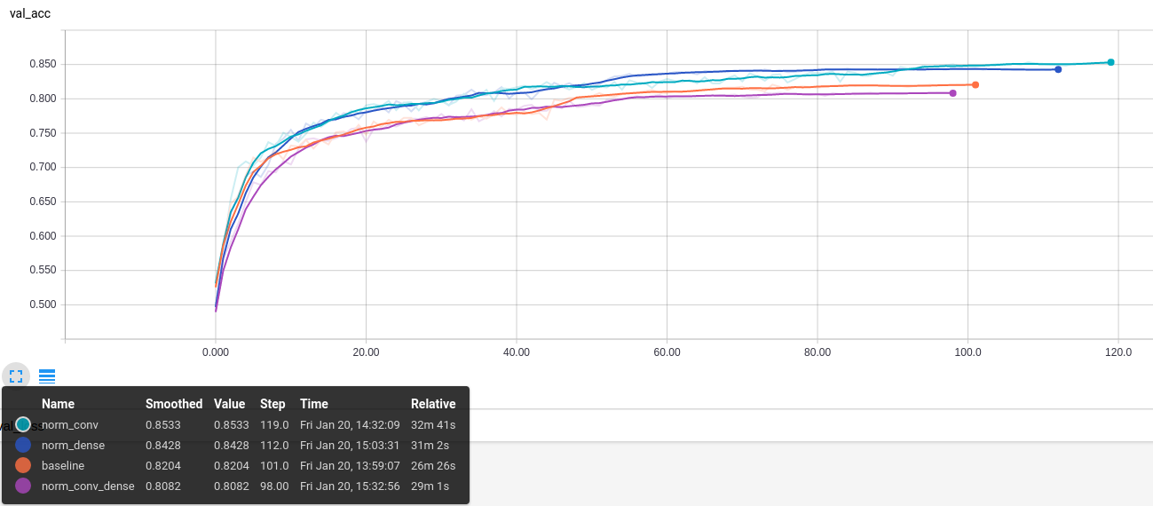
Weight normalization can be applied to both Convolutional and Dense layers. I tried all four combinations.
-
baseline: conv, dense
-
norm_conv: conv_norm, dense
-
norm_dense: conv dense_norm
-
norm_conv_dense: conv_norm, dense_norm
Test model image::alt_neural1/model.png[test_model, 300]
Discussion
Convergence graphs for all four variations are shown in fig. As hypothesized, convergence improves with internal weight normalization. More experimentation is needed to see if this holds across various models and datasets. Intriguingly, the benefits are lost when both 'Conv` and Dense layers are normalized. It is as if they 'cancel out'. I am not sure why this happens.
Additionally, the use of ReLU which effectively attenuates negative values. This limits the neuron to only communicate information when the angle between \(X\) and \(W\) lies between \([-\frac{\pi}{2}, \frac{\pi}{2}]\). Perhaps it is useful if a neuron could also communicate the lack of similarity or the inverse of weight template information. For example, the lack of a specific stripe pattern might increase the networks confidence that the output is more likely to be one cat species over another.
One way to remedy this problem might be to use an activation function that allows negative values. A quick experiment with ELU activation, however, did not result in significant improvement.
Reproducibility
The code to reproduce all the experiments in this blog is available on Github. Feel free to reuse or improve.