Ever since AlexNet was introduced in 2012, neural net research landscape fundamentally changed. With deep computational graphs, the possibilities are endless. We quickly iterated through a dizzying number of architectures such as AlexNet, VGGNet, NIN, Inception, ResNets, FractalNet, Xception, DenseNets and so on. With deep learning, architecture engineering is the new feature engineering and it clearly plays an important role in advancing the state of the art. Instead of making incremental improvements, is there a way to learn the connectivity pattern itself?
First step is to make this more concrete. Ideally, we want to learn connectivity amongst individual neurons; instead, lets simplify the problem by constraining ourselves to known layer Lego blocks (by layer Lego blocks, I mean general purpose computational layers such as Convolutional Layer, LSTM, Pooling etc.). Given a bunch of Layer Legos \(L = \{L_{1}, L_{2}, \cdots, L_{n}\}\), our task is to learn how these should be assembled. First thing that comes to mind is evolutionary search, but that is computationally prohibitive. A quicker and more elegant alternative would be to learn this by computing the gradient of architecture with respect to loss. The challenge is to make architecture itself differentiable.
Differentiable Architecture
Architecture can mean a lot of things. For now, let us constrain ourselves to connectivity patterns. Given some \(n\) layers, what is the optimal connectivity amongst them? The naive way of approaching this problem would be to try out all \(n(n-1)\) possible connection configurations[1]. There is a resnet, densenet or some other future net hidden in there.
Bruteforce search is not such a bad option. Cifar10/100 networks are quite short (relatively speaking). If you have access to huge compute, it might take a month to try out all possible connectivities. Hopefully we can extrapolate the recurring blocks and apply it to imagenet and get a new SOTA results (wishful thinking). While practical, this is a rather boring way to solve the problem. What if we can learn the connections via gradient descent? For this to work, we need a way to compute \(\frac{\partial (loss)}{\partial (connection)}\).
Connectivity is inherently binary. This is problematic for applying gradient descent because of the discontinuity. Notice the similarities with attention? We can employ reinforcement learning like hard attention or try soft attention strategy. In order to make connectivity continuous, we can make it weighted, similar to forget gate in LSTMs[2]. To bias the connectivity mostly towards 0 or 1, we can apply use sigmoid weighted connectivity. To recap, the strategy is to start out with a fully connected net where evry layer is connected to every other layer via sigmoid weighted param. The weights can be learned via backprop.
Cool. There is one slight technicality. Backward connections introduce cycles in the graph[3]. Excluding backward connections, every layer can have incoming inputs from all previous layers, which leaves us with \(\frac{n(n-1)}{2}\) possible connections. This is exactly what DenseNets do!, except that we arrived at a similar architecture with a different motivation.
Unlike DenseNets, we want the connections to be gated so that they can be pruned if needed. There are a couple of possibilities for how \(L_{i}\) is connected to \(L_{j}\).
-
Shared/Unique feature weights: We can either associate weights \(W = [w_{1}, w_{2}, \cdots, w_{f}]\) for \(L_{i}\) with \(f\) feature maps or use a single weight for all feature maps of an incoming input. Lets call this shared/unique feature weight scheme.
-
Input aggregation: For layer \(L_{j}\), we need a way to aggregate weight feature maps from previous layers. Some possibilities include:
-
DenseNet style concat: i.e, simply concatenate previous layer weighted feature maps. This has the limitation that concatenation is not viable when the size of feature maps differ. For this we can either try to pad smaller feature maps with 0’s to make them all the same size as the largest feature map or resize all feature maps to the smallest feature map by pooling/interpolation/some other form of down sampling. Both approaches have their own pros and cons. The first is computationally expensive (since convnets have to slide over larger feature maps), while the second one is lossy. I have a feeling that lossy would end up being the winner.
-
ResNet style concat: i.e., squish weighted input feature maps via max or sum. avg, prod, min dont seem like good ideas for obvious reasons. I like max better than resnet style sum, since it is equivalent to focusing on input patterns that matched with a filter (high output value) across various feature maps. A high value at some \((row, col)\) of the filter might indicate the presence of some abstract shape detected by previous convolutional layers.
-
Squeeze net style concat: Lastly, we can also try squeeze net strategy of squishing \(n\) concatenated input feature maps (after reshaping to same size via padding or down sampling) down to \(m\) feature maps where \(m \le n\).
-
Phew! That completes our setup. The idea is super simple. Start out with an fully connected network where every layer gets inputs from all the previous layers in a weighted fashion. Before weighing, we use \(sigmoid(W)\) to bias the values mostly towards 0 or 1. When trained end-end via backprop, the network should, in-principle, learn to prune unwanted connections.
We can also try doing couple of other things.
-
Take the converged connectivity pattern and try it exclusively by removing connections with small weights. If \(w = 0.002\) or something like that, we know that the network is trying really hard to get rid of that connection. So might as well see if the performance is better when we start out by removing it.
-
Examine the evolution of weights during training. Do they always converge in the same manner? If they don’t, that would be concerning.
-
Try different connection weight initialization schemes. \(w = 1\) would mean everything starts out fully connected. Alternatively we can set \(w\) from a Gaussian distribution centered around 0.5. We can try other funky things like setting initial feed forward stack \(L_{i-1}\) → \(L_{i}\) weight to 1 and rest to 0.5.
Experimental Setup
-
Layers = [Conv, Conv, MaxPool, Dropout] \(\times\) 2-3 blocks of variable feature sizes.
-
cifar10 dataset augmented with 10% random shifts along image rows/cols along with a 50% chance of horizontal flip.
-
random_seed = 1337for reproducibility. -
Training for 200 epochs, batch size of 32 using categorical cross-entropy loss with Adam optimizer.
Implementation
A quick summary of these ideas are translated into concrete implementation. A complete implementation can be found on my github.
-
Creating fully connected net. i.e, a layer is connected to all prev layer outputs. This is not as hard as it appears.
def make_fully_connected(x, layers):
    inputs = [x]
    for layer in layers:
        x = layer(x)
        inputs.append(x)
        # This is the part where we resize inputs to be of same shape and merge them in resnet or densenet style
return x-
Merging. i.e., resizing prev layer outputs to be of the same shape and concatenating them in densenet or resnet style. We also want to weigh merged outputs so that those weights can be learned during backprop. The easiest way to do this in keras is to create a custom layer[4].
import numpy as np
import tensorflow as tf

from keras import backend as K
from keras.layers import Lambda, Layer

class Connection(Layer):
    """Takes a list of inputs, resizes them to the same shape, and outputs a weighted merge.
    """
    def __init__(self, init_value=0.5, merge_mode='concat',
                 resize_interpolation=tf.image.ResizeMethod.BILINEAR,
                 shared_weights=True):
        """Creates a connection that encapsulates weighted connection of input feature maps.

        :param init_value: The init value for connection weight
        :param merge_mode: Defines how feature maps from inputs are aggregated.
        :param resize_interpolation: The downscaling interpolation to use. Instance of `tf.image.ResizeMethod`.
            Note that ResizeMethod.AREA will fail as its gradient is not yet implemented.
        :param shared_weights: True to share the same weight for all feature maps from inputs[i].
        False creates a separate weight per feature map.
        """
        self.init_value = init_value
        self.merge_mode = merge_mode
        self.resize_interpolation = resize_interpolation
        self.shared_weights = shared_weights
        super(Connection, self).__init__()

    def _ensure_same_size(self, inputs):
        """Ensures that all inputs match last input size.
        """
        # Find min (row, col) value and resize all inputs to that value.
        rows = min([K.int_shape(x)[1] for x in inputs])
        cols = min([K.int_shape(x)[2] for x in inputs])
        return [tf.image.resize_images(x, [rows, cols], self.resize_interpolation) for x in inputs]

    def _merge(self, inputs):
        """Define other merge ops like [+, X, Avg] here.
        """
        if self.merge_mode == 'concat':
            # inputs are already stacked.
            return inputs
        else:
            raise RuntimeError('mode {} is invalid'.format(self.merge_mode))

    def build(self, input_shape):
        """ Create trainable weights for this connection
        """
        # Number of trainable weights = sum of all filters in `input_shape`
        nb_filters = sum([s[3] for s in input_shape])

        # Create shared weights for all filters within an input layer.
        if self.shared_weights:
            weights = []
            for shape in input_shape:
                # Create shared weight, make nb_filter number of clones.
                shared_w = K.variable(self.init_value)
                for _ in range(shape[3]):
                    weights.append(shared_w)
            self.W = K.concatenate(weights, axis=-1)
        else:
            self.W = K.variable(np.ones(shape=nb_filters) * self.init_value)

        self._trainable_weights.append(self.W)
        super(Connection, self).build(input_shape)

    def call(self, layer_inputs, mask=None):
        # Resize all inputs to same size.
        resized_inputs = self._ensure_same_size(layer_inputs)

        # Compute sigmoid weighted inputs
        stacked = K.concatenate(resized_inputs, axis=-1)
        weighted = stacked * K.sigmoid(self.W)

        # Merge according to provided merge strategy.
        merged = self._merge(weighted)

        # Cache this for use in `get_output_shape_for`
        self._out_shape = K.int_shape(merged)
        return merged

    def get_output_shape_for(self, input_shape):
        return self._out_shape
Lets look at this step by step.
-
_ensure_same_sizecomputes smallest \((rows, cols)\) amongst all inputs and uses it to resize all inputs to be the same shape using the provided resize interpolation scheme. -
We have to define trainable weights in
buildper keras custom layer docs. We need as many weights as sum of filters across all inputs to theConnectionlayer. Weight sharing across all filters of an incoming layer can be achieved by concatenating same weight variable for all filters. -
callcomputes sigmoid weighted inputs (I tested without sigmoid, and as expected, sigmoid weighing which mostly "allows or disallows inputs" worked a lot better), merged with defined merge strategy. We can tweakinit_valueandmerge_modeto try various init strategies for weights and different merge strategies.
The fully connected net using layers defined below, followed by sequential Dense layers using the above code is shown in fig.
layers = [
	Convolution2D(32, 3, 3, border_mode='same', activation='relu', bias=False),
	Convolution2D(32, 3, 3, bias=False, activation='relu'),
	MaxPooling2D(pool_size=(2, 2)),
	Dropout(0.25),

	Convolution2D(64, 3, 3, bias=False, activation='relu', border_mode='same'),
	Convolution2D(64, 3, 3, bias=False, activation='relu'),
	MaxPooling2D(pool_size=(2, 2)),
	Dropout(0.25)
]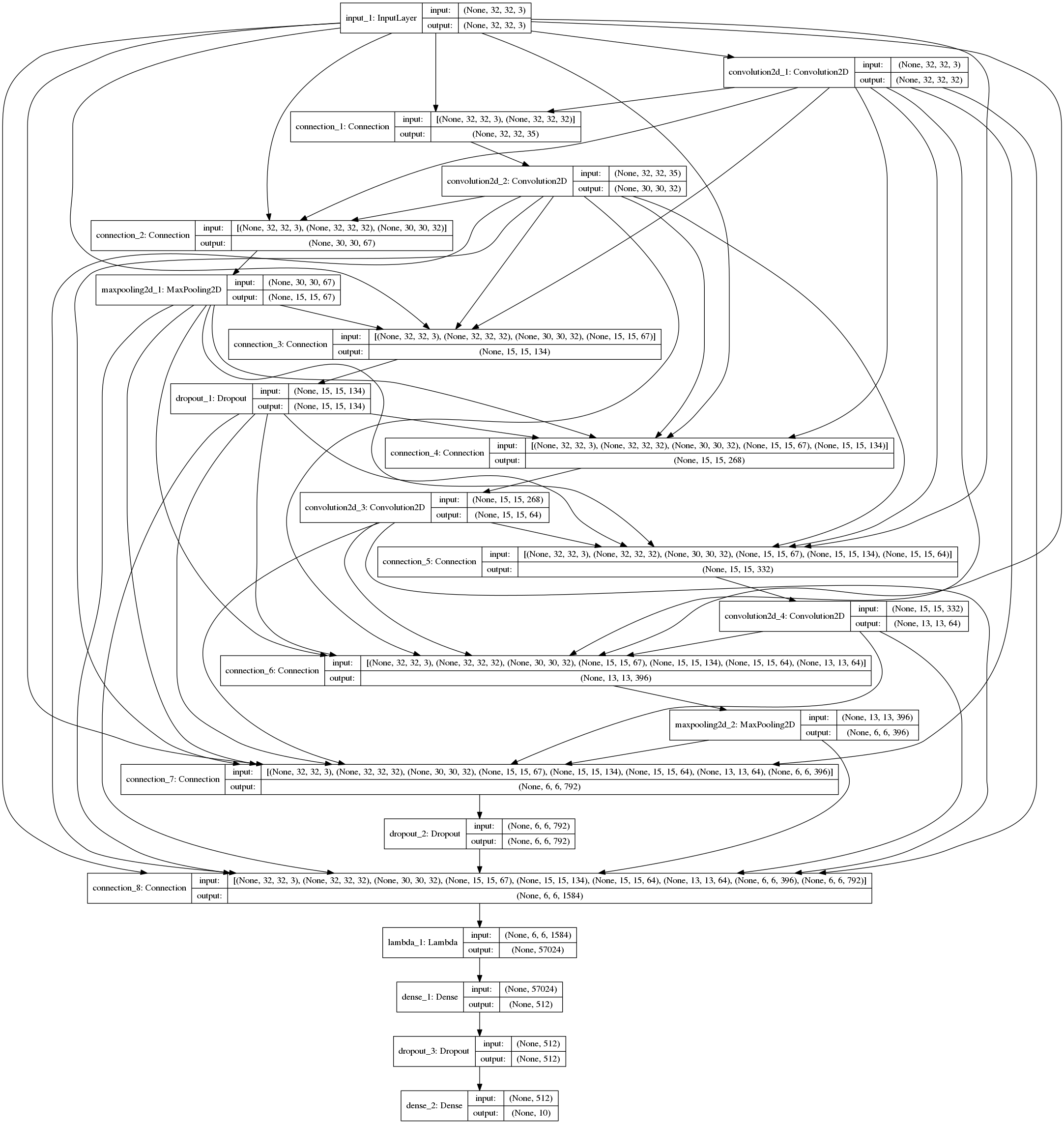
layers followed by sequential Dense layers (open in new tab or download to zoom in).Discussion
| Experimentation is still a work in progress. Check back for updates. |
Without \(sigmoid\) weighing which mostly "allows or disallows inputs", the convergence was horribly slow. All subsequent results described here used \(sigmoid\) connection weights.
Experiment1: DenseNet Style merge
In these set of experiments, activation maps from prev layers are concatenated.
Insights from initial exploration
-
Connection weight initialization scheme (init to 0, 1, 0.5) has no effect on convergence.
-
Down sampling interpolation scheme (inter_area, inter_nn, inter_bilinear, inter_bicubic) doesn’t affect the convergence significantly[5].
Evolution of connection weights (shared feature map weights)
It is definitely interesting to track how connection weights between layers evolved with training epochs. Fig 3 shows the connection weight evolution for connection_o through connection_7 (connection 0 weight 0 corresponds to input→conv2, connection 0 weight 1 corresponds to conv1→input2, and so on. Refer to fig 2 to get a complete picture).
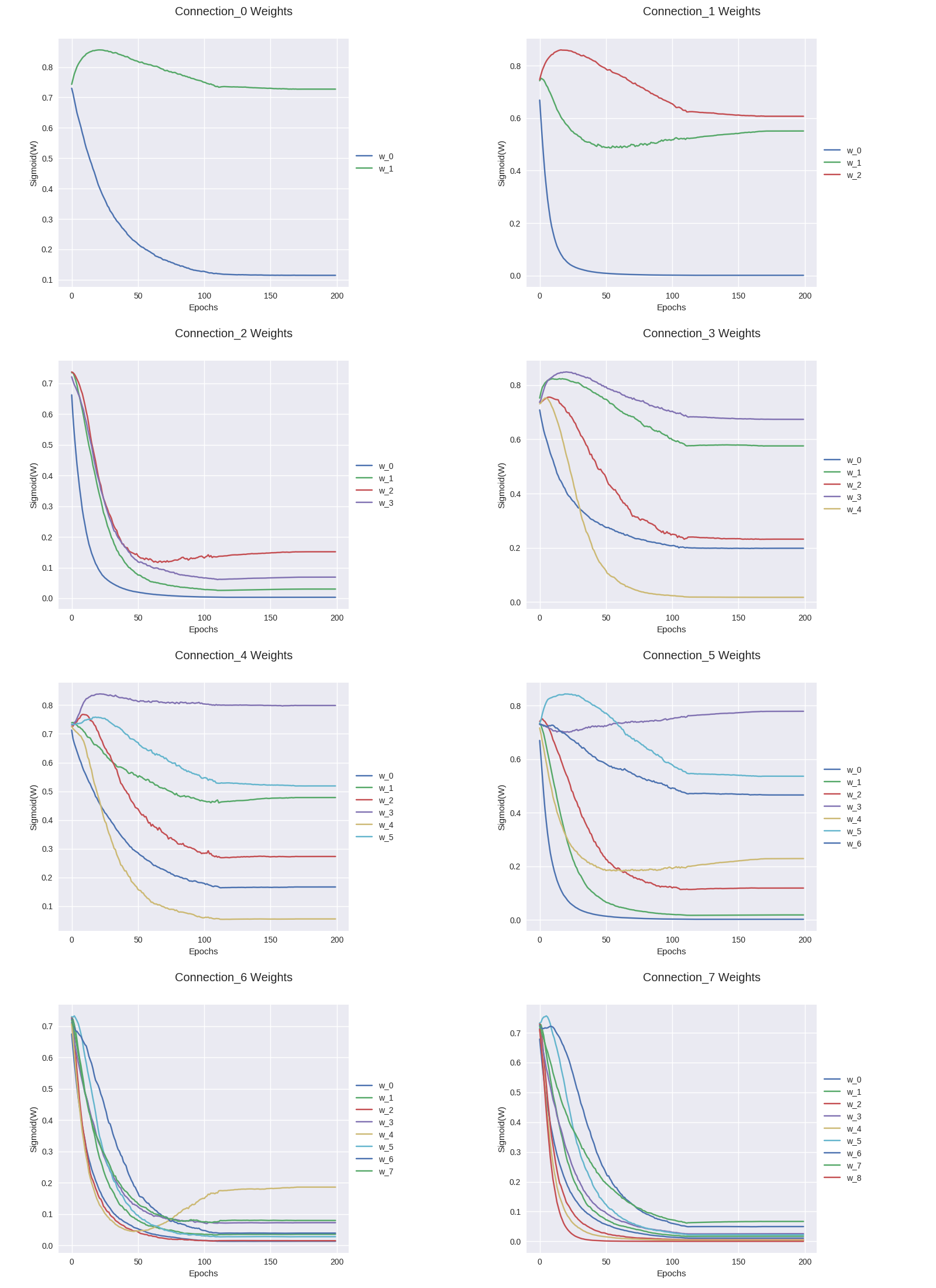
TODO: Discussion.
Evolution of connection weights (unique feature map weights)
WIP..
Reproducibility
The code to reproduce all the experiments is available on Github. Feel free to reuse or improve.